nPort RF Analysis

nPort RF Analysis embeds RF and microwave network analysis in Obsidian Markdown notes. It runs verbatim nP JavaScript on demand and retains declarative JSON blocks for safe automatic rendering. Results appear as inline SVG line charts, Smith charts, or tables.

The plugin currently supports the Obsidian desktop application. Mobile support will be declared only after it has been tested on Obsidian Mobile.

Installation

After the plugin is published in the Obsidian Community Plugin directory:

1. Open Settings → Community plugins in the vault where you want to use it.
2. Select Browse, search for nPort RF Analysis, and select Install.
3. Select Enable.

For a manual installation, download main.js, manifest.json, and styles.css from the GitHub release whose tag matches the version in manifest.json. Place the three files in:

<vault>/.obsidian/plugins/np-rf-analysis/

Restart Obsidian, then enable nPort RF Analysis under Settings → Community plugins. Plugins are installed and enabled separately for each vault.

To add the bundled material, open Settings → Community plugins → nPort RF Analysis. Select Install lessons or Install examples independently. The plugin creates nPort RF Analysis/Lessons and nPort RF Analysis/Examples, adds only missing files, and preserves existing files. When a collection shows Installed, close Settings and open its folder in the Files pane.

The 0.3.2 development source contains the complete numbered lesson sequence, converted examples, referenced SVGs, and schematic-authoring files promoted from the dedicated authoring vault. Publishing it as an Obsidian update remains a separate step.

Verbatim JavaScript

Use an npjs block for the full nP JavaScript API. The source is executed without translation after you select Run.

```npjs
var g = nP.global;
g.fList = g.fGen(100e6, 1000e6, 51);

var r1 = nP.R(25);
var l1 = nP.L(2e-9);

var network = nP.nodal(
    [r1, 1, 2],
    [l1, 2, 3],
    ['out', 1, 3]
);

var output = network.out('s11dB', 's21dB');
nP.lineChart({
    inputTable: [output],
    title: 'Network response',
    mount: '#chartDiv',
    backgroundColor: 'white'
});
```

Each block provides Run, Stop, and Reset controls:

• Run starts a fresh isolated execution and clears results from the previous run.
• Stop terminates the worker immediately and leaves results already rendered.
• Reset terminates execution and clears charts, tables, messages, and errors.

Successful results are saved as validated render instructions and restored when the note is rendered again. This lets Obsidian include charts, tables, and text results in Export to PDF without automatically rerunning JavaScript. Changing the JavaScript invalidates the saved result; run the updated block once to create a new snapshot. During PDF export, interactive controls and the security warning are hidden.

Saved results have a bounded cache lifecycle:

• Editing or deleting an npjs block removes its previous saved result.
• Deleting a note removes results owned by that note; renaming a note transfers their ownership to the new path.
• Results older than 30 days are removed by default.
• Saved-result storage is limited to 25 MB by default, with the oldest results removed first.
• Both limits are configurable under Settings → Community plugins → nPort RF Analysis.
• The settings page shows the current result count and approximate storage size and provides Clear saved results.
• The command palette also provides nPort RF Analysis: Clear saved results.
• Optional session-only mode clears saved results during a normal Obsidian quit. This is best-effort cleanup and cannot run after a crash or forced shutdown.

The cache is stored in the plugin's data.json; result data is not inserted into the Markdown note.

Inside an npjs fence, ordinary paste uses the clipboard's plain-text representation. JavaScript copied from editors such as VS Code therefore keeps its intended spaces, tabs, and line breaks without importing rich-text paragraph formatting.

In Reading view, the controls and Status: Ready appear above the complete, always-visible JavaScript source. Charts, tables, messages, and errors appear below the source.

Selectors such as mount: '#chartDiv' are resolved within that block, so existing nP development scripts can be pasted without adding HTML mount elements. nP.lineChart(), nP.smithChart(), and nP.lineTable() render in the note; all nP analysis constructors and composition functions remain available to the script.

Optional declarative JSON

Use an np block when a validated, automatically rendered analysis is preferable:

```np
{
  "frequencies": {
    "start": 100000000,
    "stop": 6000000000,
    "points": 101,
    "referenceImpedance": 50
  },
  "components": {
    "r1": { "type": "R", "value": 25 },
    "l1": { "type": "L", "value": 2e-9 }
  },
  "nodal": [
    ["r1", 1, 2],
    ["l1", 2, 3],
    ["out", 1, 3]
  ],
  "output": ["s11dB", "s21dB"],
  "view": {
    "type": "line",
    "title": "Series R-L response",
    "metricPrefix": "giga"
  }
}
```

Switch to Reading View to render the analysis.

Security model

npjs deliberately executes user-authored JavaScript, but it does not run automatically. Only select Run for code you trust.

• Execution occurs in a disposable Web Worker inside a sandboxed iframe.
• The iframe applies a Content Security Policy that denies network connections and remote resources.
• Network, browser storage, and nested-worker APIs are disabled inside the worker.
• The script receives nP, a captured console, chart/table forwarding, and a text-only document.getElementById(...).textContent compatibility shim. It does not receive Obsidian's app, vault, actual DOM, Node.js, Electron, require, or process objects.
• Stopping, resetting, unloading the block, or completing a run destroys the execution context.
• The plugin contains no telemetry, remote code loading, self-update mechanism, or access to files outside the vault.

The safe np JSON format remains available and never executes JavaScript.

Security reports may be submitted through the repository's GitHub issues. Do not include private vault contents in a report. See SECURITY.md for the supported-version and reporting policy.

Support and feedback

For questions, bug reports, and feature requests, open an issue in the GitHub repository. Do not include private vault contents, credentials, or other sensitive information.

The plugin settings page provides independent installation controls for Lessons and Examples, plus Open documentation and Report an issue buttons. The installation controls write their disclosed files only below nPort RF Analysis in the current vault and never overwrite existing files. Installed collections are opened from Obsidian's Files pane. The other two buttons open GitHub in the default browser only after you select them; the plugin makes no background network requests.

Supported features

• Frequency ranges, reference impedance, and temperature.
• R, L, C, seR, seL, seC, paR, paL, paC, Tee, Open, Short, Load, and Tlin components.
• Explicit nP.nodal() topology.
• All .out(...) suffixes: mag, dB, ang, Re, and Im.
• Line charts, Smith charts, and SVG tables.
• Light and dark theme-aware containers.
• Isolated nP global analysis settings for every block.
• Verbatim nP JavaScript with explicit Run, Stop, and Reset controls.
• Optional JSON validation without JavaScript execution.

For a Smith chart, request paired real and imaginary outputs and set view.type to smith:

"output": ["s11Re", "s11Im"],
"view": { "type": "smith", "title": "Input match" }

Local development

The prototype includes a pinned, generated nP ESM bundle under vendor/ so releases and CI are self-contained. The vendored bundle is generated from the nP 0.0.48 plugin entry and remains covered by nP's MIT license. That entry contains the complete RF, math, component, diode, chart, and table APIs, but intentionally excludes nP's obsolete browser-development helpers. The worker is bundled into main.js; the plugin does not download executable code at runtime.

Bundled learning and example content

Educational content is authored and verified in the dedicated np-rf-analysis-test-vault, then promoted into reviewable Markdown and SVG source assets in this repository. The production build embeds those source assets into main.js; users do not need the authoring vault, an AI CLI, or a network connection to create and use the bundled material.

The intended complete bundle contains Lessons 1–22, reference notes 100 and 200, the converted Examples hierarchy, and every real SVG referenced by those notes. Administrative files such as AGENTS.md are excluded. The my-circuit.svg name shown in lesson 22 is placeholder code, not a required asset.

Promotion must preserve internal paths and must verify that all intended files are present and all real SVG references resolve. Generated main.js remains ignored source output; Markdown and SVG files, the promotion procedure, and the validation tests remain reviewable in the repository. Content creation in a user's vault adds only missing files by default and does not overwrite the user's edits.

During coordinated nP development, the repositories can still be kept as siblings:

parent/
├── nP/
└── np-rf-analysis/

Build and test with:

npm install
npm run typecheck
npm test
npm run build

For manual Obsidian testing, copy or link this directory into a dedicated test vault as:

<test-vault>/.obsidian/plugins/np-rf-analysis/

Obsidian loads manifest.json, main.js, and styles.css. Do not develop against an important vault.

Complete nP API reference

The following reference is maintained from lesson 200 of the learning guide and covers the public API bundled with the versions identified below.

Version Covered

This list applies to:

• nP library: 0.0.48
• nPort RF Analysis Obsidian plugin: 0.3.2
• Reference updated: 2026-08-18

The two version numbers are independent. The plugin has its own release version and bundles a particular version of the nP library.

This reference was audited against the public export list and returned-object APIs in the nP module bundled with plugin 0.3.2. It covers every public export in nP 0.0.48; internal implementation helpers are outside its scope.

Display the bundled nP version in the console pane with:

console.log("nP version " + nP.version);

Expected console output:

[log] nP version 0.0.48

When the bundled nP version changes, re-audit the export list, signatures, defaults, returned members, and runnable examples before updating this version statement.

Constructor Conventions

Set the frequency list before calling an RF constructor:

var g = nP.global;
g.fList = g.fGen(1e9, 10e9, 11);

Unless stated otherwise:

• Resistance is in ohms.
• Inductance is in henries.
• Capacitance is in farads.
• Frequency is in hertz.
• Physical dimensions are in meters.
• Constructors use nP.global.fList, nP.global.Ro, and, when applicable, nP.global.Temp.
• RF constructors return n-port objects containing S-parameters for every active frequency.
• A displayed default is the value used when that argument or option is omitted.

In the constructor tables, Chainable: Yes means the constructor returns a two-port that can validly continue with .cas(nextTwoPort). See Method Chaining for the complete rules and examples.

Basic RLC Constructors

The uppercase short names are the preferred constructors for ordinary explicit circuit descriptions.

Constructor	Signature	Ports	Description	Chainable
nP.R()	(R = 75)	2	Series resistor.	Yes
nP.L()	(L = 5e-9)	2	Series inductor.	Yes
nP.C()	(C = 1e-12)	2	Series capacitor.	Yes
nP.seR()	(R = 75)	2	Explicitly named series resistor; equivalent role to R().	Yes
nP.seL()	(L = 5e-9)	2	Explicitly named series inductor; equivalent role to L().	Yes
nP.seC()	(C = 1e-12)	2	Explicitly named series capacitor; equivalent role to C().	Yes
nP.paR()	(R = 75)	2	Shunt resistor.	Yes
nP.paL()	(L = 5e-9)	2	Shunt inductor.	Yes
nP.paC()	(C = 1e-12)	2	Shunt capacitor.	Yes

Basic RLC example

var r1 = nP.R(75);
var l1 = nP.L(5e-9);
var c1 = nP.C(1e-12);

Basic RLC Symbols

This visual catalog uses the preferred explicit constructors.

Canonical RLC symbols

Constructor	Canonical symbol
nP.R()
nP.L()
nP.C()

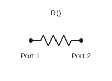
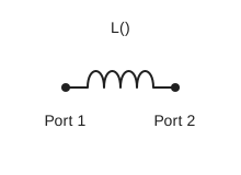
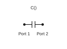
Combined RLC Constructors

The combined-constructor names contain two topology prefixes:

• The first se or pa says whether the completed equivalent impedance is placed in the two-port's series path or as a shunt branch.
• The second Se or Pa says whether the R, L, and C elements are internally combined in series or parallel.

For example, sePaRC() places a parallel-RC equivalent impedance in the two-port's series path. paSeRC() places a series-RC branch in shunt.

Internally Series Elements

Constructor	Signature	Ports	Description	Chainable
nP.seSeRL()	(R = 75, L = 5e-9)	2	Series-RL impedance in the two-port series path.	Yes
nP.paSeRL()	(R = 75, L = 5e-9)	2	Series-RL impedance as a shunt branch.	Yes
nP.seSeRC()	(R = 75, C = 1e-12)	2	Series-RC impedance in the two-port series path.	Yes
nP.paSeRC()	(R = 75, C = 1e-12)	2	Series-RC impedance as a shunt branch.	Yes
nP.seSeLC()	(L = 5e-9, C = 1e-12)	2	Series-LC impedance in the two-port series path.	Yes
nP.paSeLC()	(L = 5e-9, C = 1e-12)	2	Series-LC impedance as a shunt branch.	Yes
nP.seSeRLC()	(R = 75, L = 5e-9, C = 1e-12)	2	Series-RLC impedance in the two-port series path.	Yes
nP.paSeRLC()	(R = 75, L = 5e-9, C = 1e-12)	2	Series-RLC impedance as a shunt branch.	Yes

Internally Parallel Elements

Constructor	Signature	Ports	Description	Chainable
nP.sePaRL()	(R = 75, L = 5e-9)	2	Parallel-RL impedance in the two-port series path.	Yes
nP.paPaRL()	(R = 75, L = 5e-9)	2	Parallel-RL impedance as a shunt branch.	Yes
nP.sePaRC()	(R = 75, C = 1e-12)	2	Parallel-RC impedance in the two-port series path.	Yes
nP.paPaRC()	(R = 75, C = 1e-12)	2	Parallel-RC impedance as a shunt branch.	Yes
nP.sePaLC()	(L = 5e-9, C = 1e-12)	2	Parallel-LC impedance in the two-port series path.	Yes
nP.paPaLC()	(L = 5e-9, C = 1e-12)	2	Parallel-LC impedance as a shunt branch.	Yes
nP.sePaRLC()	(R = 75, L = 5e-9, C = 1e-12)	2	Parallel-RLC impedance in the two-port series path.	Yes
nP.paPaRLC()	(R = 75, L = 5e-9, C = 1e-12)	2	Parallel-RLC impedance as a shunt branch.	Yes

For instructional circuits and arbitrary topologies, explicit R(), L(), and C() components connected with nP.nodal() usually make the circuit easier to read.

The combined RLC constructors intentionally have no symbol-library entries. Their internal combinations are clearer when drawn and coded as explicit components connected with nP.nodal().

Transformer Constructors

Constructor	Signature	Ports	Description	Chainable
nP.trf()	(N = 0.5)	2	Ideal two-port transformer model.	Yes
nP.trf4Port()	(N = 0.5)	4	Ideal four-port transformer model.	No

N is the transformer turns-ratio parameter used by the model.

Canonical transformer symbols

Constructor	Canonical symbol
nP.trf()
nP.trf4Port()

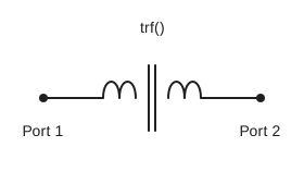
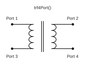
For trf4Port(), ports 1 and 3 are the primary pair and ports 2 and 4 are the secondary pair.

Ideal Components and Junctions

Ideal component names begin with an uppercase letter.

Constructor	Signature	Ports	Description	Chainable
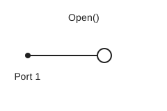
nP.Open()	()	1	Ideal open circuit.	No
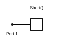
nP.Short()	()	1	Ideal short circuit.	No
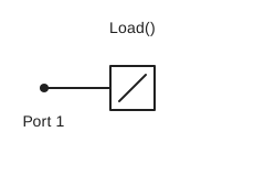
nP.Load()	()	1	Ideal matched load.	No
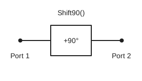
nP.Shift90()	()	2	Matched lossless two-port with +90° through phase.	Yes
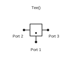
nP.Tee()	()	3	Ideal three-port junction.	No
nP.seriesTee()	()	3	Ideal series junction: ports 1 and 2 form the through path; port 3 accepts a one-port series branch.	No
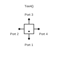
nP.Tee4()	()	4	Ideal four-port junction.	No
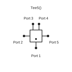
nP.Tee5()	()	5	Ideal five-port junction.	No
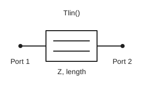
nP.Tlin()	(Z = 60, Length = 0.0127)	2	Ideal lossless transmission line.	Yes
nP.Tclin()	(Zoe = 100, Zoo = 30, Length = 0.037338)	4	Ideal lossless coupled transmission line.	No

For Tlin(), Z is characteristic impedance and Length is physical length. For Tclin(), Zoe and Zoo are the even- and odd-mode impedances.

Canonical ideal-component symbols

Constructor	Canonical symbol
nP.Open()
nP.Short()
nP.Load()
nP.Shift90()
nP.Tee()
nP.Tee4()
nP.Tee5()
nP.Tlin()
nP.Tclin()

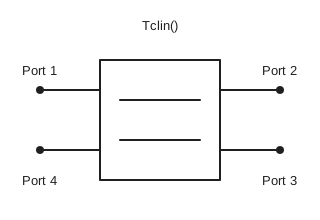
Coupled-line ports are numbered clockwise:

port 1  ─── coupled line ─── port 2
port 4  ─── coupled line ─── port 3

Physical Transmission-Media Constructors

Physical transmission-media constructors are organized by their modeling family. The current library provides the microstrip mlin family. Future stripline, coaxial, and waveguide families can be added here as peer sections without being grouped under a JavaScript argument style.

Microstrip: the mlin Constructor Family

All current microstrip component implementations belong to the mlin source family. Their public constructor names are lowercase, and physical dimensions are in meters.

Constructor	Signature	Ports	Description	Chainable
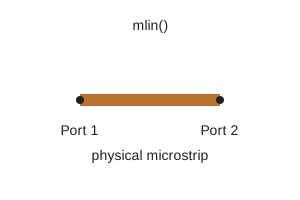
nP.mlin()	(Width, Height, Length, Thickness, er, rho, tand, roughnessRms)	2	Physical microstrip transmission line.	Yes
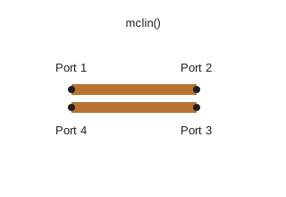
nP.mclin()	(Width, Space, Height, Thickness, Length, er, rho, tand, roughnessRms)	4	Physical coupled microstrip line.	No
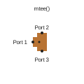
nP.mtee()	(commonWidth, branch1Width, branch2Width, Height, Thickness, er, rho, tand, roughnessRms)	3	Physical microstrip tee junction.	No
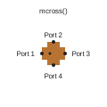
nP.mcross()	(options)	4	Physical microstrip cross junction.	No
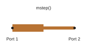
nP.mstep()	(options)	2	Physical microstrip width step.	Yes
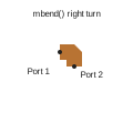
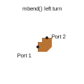
nP.mbend()	(options)	2	Physical microstrip bend.	Yes
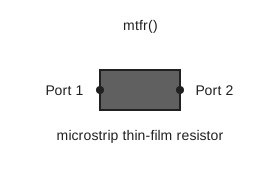
nP.mtfr()	(options)	2	Distributed microstrip thin-film resistor.	Yes
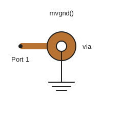
nP.mvgnd()	(options)	1	Physical via-to-ground model.	No
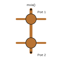
nP.mvia()	(options)	2	Physical via transition between conductor layers.	Yes

Microstrip signatures, options, and mtee() defaults Positional-argument constructors

nP.mlin(
    Width = 0.023 * 0.0254,
    Height = 0.025 * 0.0254,
    Length = 0.5 * 0.0254,
    Thickness = 0.0000125 * 0.0254,
    er = 10,
    rho = 1,
    tand = 0.001,
    roughnessRms = 0
)

nP.mclin(
    Width = 19.1155 * 0.001 * 0.0254,
    Space = 5.82185 * 0.001 * 0.0254,
    Height = 25 * 0.001 * 0.0254,
    Thickness = 0.0000125 * 0.0254,
    Length = 719.794 * 0.001 * 0.0254,
    er = 10,
    rho = 1,
    tand = 0.001,
    roughnessRms = 0
)

For mlin() and mclin(), rho is a resistivity multiplier relative to copper. A value of 0 disables conductor loss. mclin() uses the same clockwise port convention as Tclin().

Options-object defaults

nP.mtee(
    0.023 * 0.0254,
    0.023 * 0.0254,
    0.023 * 0.0254,
    0.025 * 0.0254,
    0.0000125 * 0.0254,
    10,
    1,
    0.001,
    0
)

nP.mcross({
    leftWidth: 0.023 * 0.0254,
    topWidth: 0.023 * 0.0254,
    rightWidth: 0.023 * 0.0254,
    bottomWidth: 0.023 * 0.0254,
    Height: 0.025 * 0.0254,
    Thickness: 0.0000125 * 0.0254,
    er: 10, rho: 1, tand: 0.001, roughnessRms: 0
})

nP.mstep({
    width1: 0.046 * 0.0254,
    width2: 0.023 * 0.0254,
    Height: 0.025 * 0.0254,
    Thickness: 0.0000125 * 0.0254,
    er: 10, rho: 1, tand: 0.001, roughnessRms: 0
})

nP.mbend({
    Width: 0.023 * 0.0254,
    miterLength: 0,
    Height: 0.025 * 0.0254,
    Thickness: 0.0000125 * 0.0254,
    er: 10, rho: 1, tand: 0.001, roughnessRms: 0
})

nP.mtfr({
    ohmsPerSquare: 50,
    Width: 10 * 0.001 * 0.0254,
    Length: 10 * 0.001 * 0.0254,
    Height: 0.025 * 0.0254,
    Thickness: 0.0000125 * 0.0254,
    er: 10,
    tand: 0.001,
    temperatureCoefficient: 0,
    temperatureReference: 25,
    sections: undefined
})

nP.mvgnd({
    Diameter: 100e-6,
    Height: 0.025 * 0.0254,
    Thickness: 0.0000125 * 0.0254,
    rho: 1.72e-8
})

nP.mvia({
    Diameter: 100e-6,
    connectionHeight: 0.025 * 0.0254,
    Thickness: 0.0000125 * 0.0254,
    rho: 1.72e-8,
    er: 10,
    padDiameter: 0,
    antipadDiameter: 0,
    topPadHeight: 0,
    bottomPadHeight: 0,
    topStubLength: 0,
    bottomStubLength: 0
})

mvgnd() and mvia() use absolute conductor resistivity in Ω·m, not the relative rho multiplier used by mlin() and mclin(). For mtfr(), sections = automatic means nP selects Math.min(200, Math.max(10, Math.ceil((Length / Width) * 10))); an explicitly supplied value is floored and clamped to at least 1.

nP.mtee(commonWidth, branch1Width, branch2Width, Height, Thickness, er, rho, tand, roughnessRms)

mtee() calculates a physical three-port junction discontinuity from the three arm widths and substrate geometry. Omitted positional arguments use the defaults below. The earlier options-object form remains supported for backward compatibility.

Parameter	Default	Meaning
commonWidth	0.023 * 0.0254 m = 0.5842 mm	Width of the common arm connected to port 1.
branch1Width	0.023 * 0.0254 m = 0.5842 mm	Width of the first branch connected to port 2.
branch2Width	0.023 * 0.0254 m = 0.5842 mm	Width of the second branch connected to port 3.
Height	0.025 * 0.0254 m = 0.635 mm	Substrate height between the trace and its reference plane.
Thickness	0.0000125 * 0.0254 m = 0.3175 µm	Metal thickness.
er	10	Relative permittivity, also called the dielectric constant.
rho	1	Conductor-resistivity multiplier relative to copper.
tand	0.001	Dielectric loss tangent.
roughnessRms	0 m	RMS conductor-surface roughness; zero represents a smooth conductor.

Ports: port 1 is the common arm, port 2 is branch 1, and port 3 is branch 2.

JavaScript capitalization matters: use Height and Thickness with uppercase first letters. Set nP.global.fList before constructing the tee.

In nP 0.0.48, the tee-junction calculation uses the three widths, Height, Thickness, and er. It records rho, tand, and roughnessRms in .microstrip, but those parameters do not add loss inside the junction model. Connected mlin() sections model their own transmission-line losses.

The physical constructors expose model metadata in addition to the ordinary n-port members:

Constructors	Additional returned member
mlin, mclin, mtee, mcross, mstep, mbend, mvgnd, mvia	.microstrip, containing input geometry and model-specific calculated data.
mtfr	.filmResistor, containing geometry, resistance, section count, and temperature data.
mtee, mcross	.Ct, the junction capacitance also recorded inside .microstrip.

mtee(), mcross(), mstep(), and mbend() are discontinuity models rather than finite-length lossy lines. In nP 0.0.48, their rho, tand, and roughnessRms parameters or options are retained as metadata but do not add conductor, dielectric, or roughness loss to the discontinuity itself.

mlin Family Symbols

Canonical microstrip symbols

Constructor	Canonical symbol
nP.mlin()
nP.mclin()
nP.mtee()
nP.mcross()
nP.mstep()
nP.mbend() right turn
nP.mbend() left turn
nP.mtfr()
nP.mvgnd()
nP.mvia()

Diode Constructor

Constructor	Signature	Ports	Description	Chainable
nP.diode1N4148()	(options)	2	Small-signal RF diode model with Shockley DC I-V behavior.	Yes

The returned object is an n-port and also provides:

• .diode for model parameters, bias results, and model provenance.
• .ivTable(start, stop, points) for a DC voltage/current table.

Diode options

Option	Default	Meaning
is	2.75e-11 A	Saturation current.
n	2	Emission coefficient.
rs	0.568 Ω	Series resistance.
cj0	4e-12 F	Zero-bias junction capacitance.
vj	0.75 V	Junction potential.
m	0.5	Junction grading coefficient.
tt	4e-9 s	Transit time.
leakageResistance	4e9 Ω	Parallel leakage resistance.
breakdownVoltage	100 V	Reverse-breakdown voltage magnitude.
breakdownCurrent	100e-6 A	Breakdown-current scale.
breakdownSoftness	2 V	Exponential breakdown-voltage scale.
biasVoltage	0 V	DC bias used for the RF small-signal model.
temperatureK	nP.global.Temp	Junction temperature in kelvins.
ivStart	-110 V	Default starting voltage for .ivTable().
ivStop	1 V	Default stopping voltage for .ivTable().
ivPoints	401	Default number of .ivTable() rows, excluding the header.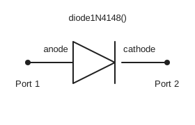

Low-Pass Network Constructor

Constructor	Signature	Ports	Description	Chainable
nP.lpfGen()	(filt = defaultFilter)	2	Low-pass two-port synthesized from an alternating termination/component value array.	Yes

New instructional examples should normally show the individual components and their nP.nodal() connections when circuit topology matters.

The default filter array is:

[50, 1.641818746502858e-11, 4.565360855435164e-8, 1.6418187465028578e-11, 50]

lpfGen() removes the first and last termination values from the supplied filt array with shift() and pop(). Pass filt.slice() when the caller must preserve the original array:

var filter = nP.lpfGen(filterValues.slice());

Chebyshev Low-Pass Design Helpers

These helpers calculate the section count, normalized prototype values, and physical component values used to build a Chebyshev low-pass network:

Helper	Signature	Returns	Chainable
nP.chebyLPNsec()	(passFreq = 0.2, rejFreq = 1.5, ripple = 0.1, rejection = 30)	Required integer number of filter sections.	No
nP.chebyLPgk()	(n = 3, ripple = 0.1)	JavaScript array containing the normalized g values, including both terminations.	No
nP.chebyLPLCs()	(cheby = defaultPrototype, maxPassFrequency = 0.2e9, zo = 50)	JavaScript array containing the source termination, alternating capacitor and inductor values, and load termination.	No

For chebyLPNsec(), passFreq and rejFreq must use the same units because their ratio determines the normalized stopband frequency. ripple and rejection are in decibels. For chebyLPLCs(), maxPassFrequency is in hertz and zo is in ohms.

The chebyLPLCs() default prototype is:

[1, 1.0315851425078764, 1.1474003299537219, 1.0315851425078761, 1]

The normal design sequence is:

1. Use chebyLPNsec() to determine the required number of sections.
2. Pass that section count to chebyLPgk() to calculate the normalized prototype.
3. Pass the prototype to chebyLPLCs() to scale it to frequency and impedance.
4. Pass the resulting component array to lpfGen() to create the two-port.

Chebyshev low-pass design sequence

var g = nP.global;
g.fList = g.fGen(0.01e9, 1.5e9, 101);

var sections = nP.chebyLPNsec(0.2e9, 1.5e9, 0.1, 30);
var prototype = nP.chebyLPgk(sections, 0.1);
var filterValues = nP.chebyLPLCs(prototype, 0.2e9, 50);
var filter = nP.lpfGen(filterValues);

console.log("sections = " + sections);
console.log(filter.out('s11dB', 's21dB'));

Canonical synthesized-network symbol Because lpfGen() synthesizes a complete network rather than one primitive component, its library drawing is a labeled network block.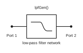

Connecting n-Port Objects

These functions combine objects returned by the constructors:

Function	Purpose
nP.nodal(...connections)	Connects arbitrary n-port objects by numbered nodes and declares external ports with ['out', ...].
nP.cascade(...nPorts)	Cascades two-port objects in order.

Every returned n-port exposes .cas(nextTwoPort), but it is valid only when both objects are two-ports with compatible frequency grids and reference impedances.

Methods on Returned n-Port Objects

The public constructors return objects with these fields and methods:

Member	Returns	Purpose
.spars	Array	S-parameter rows shaped as [frequency, s11, s12, ..., s1n, s21, ..., snn].
.global	Object	The analysis settings associated with the object.
.setspars(rows)	undefined	Replaces the S-parameter rows.
.getspars()	Array	Returns the S-parameter rows.
.setglobal(settings)	undefined	Associates global settings with the object.
.getglobal()	Object	Returns the associated global settings.
.cas(nextTwoPort)	n-port	Cascades this two-port with another two-port and returns a new two-port.
.out(...selections)	Array	Returns a numeric display table.
.outTable(...selections)	Array	Returns the same numeric output-table shape as .out().

An output selection has the case-sensitive form sijSuffix, where i is the response port, j is the excited port, and both must exist on the n-port. Valid suffixes are mag, dB, ang, Re, and Im; ang is returned in degrees. For example, s21dB is the magnitude in decibels at port 2 from excitation at port 1.

.out() selection example

var table = network.out(
    's11dB',
    's21dB',
    's11Re',
    's11Im'
);

The internal base constructor is not exported as nP.nPort(). Users create n-port objects through the public RF constructors listed above.

The library does not resample or reconcile networks during .cas(), cascade(), or nodal(). All participating objects must already have the same number and ordering of frequency points and compatible reference impedance.

Method Chaining

Method chaining means calling a method on the object returned by the preceding method:

var result = firstObject
    .firstMethod()
    .secondMethod()
    .thirdMethod();

nP supports method chaining on three object families:

Object family	What continues the chain	What ends the chain
Two-port n-port	.cas(nextTwoPort) returns a new two-port.	.out(), .outTable(), .getspars(), and .getglobal() return data rather than an n-port.
Complex number	Object-returning setters, arithmetic, copying, and complex hyperbolic methods.	Numeric accessors, magnitude, angle, and decibel methods return numbers.
Matrix	Every public Matrix method returns a Matrix object.	Reading the public .m field returns the underlying two-dimensional array.

Two-Port n-Port Chaining

The .cas() method is the source of RF-network method chaining. It connects two two-ports in cascade and returns a new two-port, so another .cas() can follow it.

These public constructors return two-ports that can participate in a .cas() chain:

Family	Chainable two-port constructors
Basic RLC	R, L, C, seR, seL, seC, paR, paL, paC
Internally series RLC	seSeRL, paSeRL, seSeRC, paSeRC, seSeLC, paSeLC, seSeRLC, paSeRLC
Internally parallel RLC	sePaRL, paPaRL, sePaRC, paPaRC, sePaLC, paPaLC, sePaRLC, paPaRLC
Transformer	trf
Ideal transmission components	Shift90, Tlin
Physical microstrip	mlin, mstep, mbend, mtfr, mvia
Other	diode1N4148, lpfGen

One-port and multiport objects cannot validly participate in .cas(). This excludes Open, Short, Load, Tee, Tee4, Tee5, trf4Port, Tclin, mclin, mtee, mcross, and mvgnd.

nP.cascade(...) and nP.nodal(...) are standalone functions, not chainable methods:

• nP.cascade(a, b, c) is a convenience function that repeatedly applies .cas().
• nP.nodal(...) solves an arbitrary node-connected topology.
• If nP.nodal(...) declares exactly two external ports, its returned two-port can begin a later .cas() chain.

Before cascading, make sure every object uses compatible nP.global.fList and nP.global.Ro values.

Two-port method chaining

var g = nP.global;
g.fList = g.fGen(1e9, 10e9, 11);

var network = nP.R(25)
    .cas(nP.L(5e-9))
    .cas(nP.C(1e-12));

var output = network.out('s11dB', 's21dB');
console.log(output);

Complex-Number Chaining

These methods return a complex object, so another complex method can follow:

Behavior	Chainable methods
Mutate and return the same object	.set(), .setR(), .setI()
Return a new complex object	.add(), .sub(), .mul(), .div(), .inv(), .neg(), .copy(), .sinhCplx(), .coshCplx()

These methods return an ordinary number and therefore end the complex-object chain:

Returned number	Chain-ending methods
Real or imaginary part	.getR(), .getI()
Magnitude or angle	.mag(), .ang()
Decibel value	.mag10dB(), .mag20dB()

Complex-number method chaining

var result = nP.complex(3, 4)
    .add(nP.complex(1, -2))
    .mul(nP.complex(2, 0))
    .inv();

console.log(result);
console.log("magnitude = " + result.mag());

The final .mag() returns a number. A complex method such as .add() cannot follow it.

Matrix Chaining

Every public Matrix method returns a Matrix object:

Behavior	Chainable Matrix methods
Set, create, or copy	.set(), .dimension(), .copyMatrix()
Real-matrix operations	.add(), .sub(), .mul(), .solveGaussFB(), .invert()
Complex-matrix operations	.addCplx(), .subCplx(), .mulCplx(), .solveGaussFBCplx(), .invertCplx()

Use the real methods when every entry is a JavaScript number. Use the Cplx methods when entries are nP.complex() objects. Matrix dimensions must be compatible with the requested operation.

Real-matrix method chaining

var identity = nP.matrix([
    [1, 0],
    [0, 1]
]);

var result = nP.matrix([
    [2, 0],
    [0, 2]
])
    .add(identity)
    .mul(identity)
    .invert();

console.log(result.m);

Accessing .m returns the underlying two-dimensional JavaScript array and ends the Matrix-object chain.

Complex Numbers

Create a complex number with:

var z = nP.complex(real, imaginary);

Example:

var z1 = nP.complex(3, 4);

The real and imaginary values are available as public numeric fields .x and .y.

In these tables, Chainable: Yes means the method returns a complex object that supports another complex method.

Complex Accessors and Mutators

Method	Purpose	Chainable
.set(real, imaginary)	Mutates both parts and returns the same object. Normally used internally by nP.complex().	Yes
.getR()	Returns the real part.	No
.getI()	Returns the imaginary part.	No
.setR(value)	Mutates the real part and returns the same object.	Yes
.setI(value)	Mutates the imaginary part and returns the same object.	Yes

Complex Arithmetic

These methods return new complex objects rather than changing the original value:

Method	Purpose	Chainable
.add(z)	Addition.	Yes
.sub(z)	Subtraction.	Yes
.mul(z)	Multiplication.	Yes
.div(z)	Division.	Yes
.inv()	Multiplicative inverse.	Yes
.neg()	Additive inverse.	Yes
.copy()	Independent copy.	Yes

Complex Magnitude, Angle, and Hyperbolic Functions

Method	Purpose	Chainable
.mag()	Magnitude.	No
.ang()	Phase angle in degrees.	No
.mag10dB()	10 log10 of the magnitude.	No
.mag20dB()	20 log10 of the magnitude.	No
.sinhCplx()	Complex hyperbolic sine.	Yes
.coshCplx()	Complex hyperbolic cosine.	Yes

Complex-number example

var z1 = nP.complex(3, 4);
var z2 = nP.complex(1, -2);

console.log("magnitude = " + z1.mag());
console.log("angle = " + z1.ang());
console.log(z1.add(z2));

Matrices

Create a matrix from a two-dimensional JavaScript array:

var a = nP.matrix([
    [1, 2],
    [3, 4]
]);

The two-dimensional array is available in the public .m field.

In these tables, Chainable: Yes means the function or method returns a Matrix object. Functions that return a plain JavaScript array are marked No.

Matrix operations assume nonempty rectangular arrays with compatible dimensions:

• .add(), .sub(), .addCplx(), and .subCplx() require equal dimensions.
• .mul() and .mulCplx() require the left column count to equal the right row count.
• .invert() and .invertCplx() require a square, nonsingular matrix.
• .solveGaussFB() and .solveGaussFBCplx() expect an augmented system with n rows and n + 1 columns and return the solution as an n × 1 Matrix.

nP 0.0.48 does not perform comprehensive dimension, shape, or singularity validation before these calculations. Verify inputs before relying on a result.

Matrix Construction Helpers

Function or method	Purpose	Chainable
nP.matrix(array2d)	Creates a matrix object from a two-dimensional array.	Yes
nP.dim(rows, cols, initial)	Creates a two-dimensional array filled with an initial value.	No
nP.dup(array2d)	Duplicates the row arrays of a two-dimensional array.	No
.set(array2d)	Replaces .m and returns the same matrix object. Normally used internally by nP.matrix().	Yes
.dimension(rows, cols, initial)	Creates a matrix object with the requested dimensions.	Yes
.copyMatrix()	Returns a copied matrix object.	Yes

Real Matrix Methods

Use these when every entry is a JavaScript number:

Method	Purpose	Chainable
.add(matrixB)	Matrix addition.	Yes
.sub(matrixB)	Matrix subtraction.	Yes
.mul(matrixB)	Matrix multiplication.	Yes
.solveGaussFB()	Solves a real augmented matrix and returns the solution column.	Yes
.invert()	Matrix inverse.	Yes

Complex Matrix Methods

Use these when the entries are nP.complex() objects:

Method	Purpose	Chainable
.addCplx(matrixB)	Complex matrix addition.	Yes
.subCplx(matrixB)	Complex matrix subtraction.	Yes
.mulCplx(matrixB)	Complex matrix multiplication.	Yes
.solveGaussFBCplx()	Solves a complex augmented matrix and returns the solution column.	Yes
.invertCplx()	Complex matrix inverse.	Yes

The solving and inversion methods operate on duplicated data and return new matrix objects. They do not intentionally overwrite the caller's matrix.

Matrix-inversion example

var a = nP.matrix([
    [1, 2],
    [3, 4]
]);

var inverse = a.invert();

console.log(inverse.m);

Display Functions and Their Returned APIs

nP.lineChart(), nP.lineTable(), and nP.smithChart() return small API objects after rendering their display. Each API provides:

• DOM or SVG element handles for advanced inspection or customization.
• Setter functions that apply styles to selected parts of the display.

Display function	Element handles	Style setters	API object chainable
nP.lineChart(options)	12	12	No
nP.lineTable(options)	7	5	No
nP.smithChart(options)	9	5	No

A style setter accepts either:

var style = { fill: "red", fontStyle: "italic" };

or a CSS declaration string:

var style = "fill:red; font-style:italic;";

The setters return undefined, not the API object. Call them separately rather than chaining them.

lineChart() returned API Element handles

Member	Returned element
.container	Display container element.
.svg	Root SVG element.
.chartBackground	Chart-background element.
.plotBorder	Plot-border element.
.txtChartTitle	Chart-title text element.
.txtXAxisTitle	X-axis-title text element.
.txtYAxisTitle	Y-axis-title text element.
.txtChartLabels	Array of trace-label text elements.
.xAxisGroup	X-axis SVG group.
.yAxisGroup	Y-axis SVG group.
.xGridGroup	X-grid SVG group.
.yGridGroup	Y-grid SVG group.

Style setters

Setter	Styles
.setTxtChartTitleStyle(style)	Chart-title text.
.setChartBackgroundStyle(style)	Chart background.
.setPlotBorderStyle(style)	Plot border.
.setTxtXAxisTitleStyle(style)	X-axis-title text.
.setTxtXAxisNumbersStyle(style)	X-axis tick-number text.
.setXAxisLineStyle(style)	X-axis path and tick lines.
.setXGridLineStyle(style)	Vertical grid lines.
.setTxtYAxisTitleStyle(style)	Y-axis-title text.
.setTxtYAxisNumbersStyle(style)	Y-axis tick-number text.
.setYAxisLineStyle(style)	Y-axis path and tick lines.
.setYGridLineStyle(style)	Horizontal grid lines.
.setTxtChartLabelsStyle(style)	Trace-label text.

lineTable() returned API Element handles

Member	Returned element
.container	Display container element.
.svg	Root SVG element.
.tableBackground	Table-background element.
.tableBorder	Outer table-border element.
.txtTableTitle	Table-title text element.
.txtHeaders	Array of header text elements.
.txtData	Array of data-cell text elements.

Style setters

Setter	Styles
.setTxtTableTitleStyle(style)	Table-title text.
.setTableBackgroundStyle(style)	Table background.
.setTableBorderStyle(style)	Outer table border.
.setTxtTableHeadersStyle(style)	Header text.
.setTxtTableDataStyle(style)	Data-cell text.

smithChart() returned API Element handles

Member	Returned element
.container	Display container element.
.svg	Root SVG element.
.chartBackground	Chart-background element.
.txtChartTitle	Chart-title text element.
.unitCircle	Smith-chart unit-circle element.
.smithGridGroup	Smith-grid SVG group.
.traceGroup	Trace SVG group.
.labelGroup	Trace-label SVG group.
.txtChartLabels	Array of trace-label text elements.

Style setters

Setter	Styles
.setTxtChartTitleStyle(style)	Chart-title text.
.setChartBackgroundStyle(style)	Chart background.
.setUnitCircleStyle(style)	Smith-chart unit circle.
.setSmithGridStyle(style)	Smith-chart grid circles and lines.
.setTxtChartLabelsStyle(style)	Trace-label text.

Display API styling

var g = nP.global;
g.fList = g.fGen(1e9, 10e9, 11);

var output = nP.R(25).out('s11dB', 's21dB');
var chartApi = nP.lineChart({
    inputTable: [output],
    chartTitle: "Styled resistor output"
});

chartApi.setTxtChartTitleStyle({
    fill: "darkred",
    fontStyle: "italic"
});

chartApi.setPlotBorderStyle("stroke:darkred; stroke-width:2;");

The element handles are an advanced escape hatch. Prefer display options and the returned style setters for ordinary customization.

Related Public APIs

The same nP 0.0.48 bundle also exports these global settings:

Member	Initial value or signature	Purpose
nP.global.fList	[2e9]	Active frequency list in hertz.
nP.global.Ro	50	Reference impedance in ohms.
nP.global.Temp	293	Analysis temperature in kelvins.
nP.global.fGen()	(fStart, fStop, points)	Returns a linearly spaced frequency array including both endpoints. Use at least two points.
nP.version	"0.0.48"	Bundled nP library version string.

nP.log(input) is also exported, but it is a legacy browser-page helper that looks for an older page-level output element. Inside an Obsidian npjs block, use console.log(input) so the message appears in that block's console pane.

Return to the start of the learning guide, or open the display-options lesson.